
Ch. 45 Projective Geometry (4) 
There is a useful technique for treating infinity  . We use what is called homogeneous coordinates. Equations of a straight line, a quadratic curve, and the like are expressed in the same degree.
Here we make Kelin's disk out of a real sphere (sphere with radius of real number) and imaginary sphere (sphere with radius of imaginary number). And we will come to the story that invisible imaginary sphere appears in our site.
The homogeneous coordinate is expressed with three letters  ,
,  ,
,  (pronounced Xi, Eta, Zeta) instead of x, y. The number of letters are three but it is certainly for a plane. The conversion between homogeneous coordinates and ordinary coordinates (non-homogeneous) is
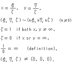 Symbol "
 " means equivalence.
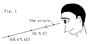 In Fig. 1 two points (, , ) and (k, k, k) are eqivalent for a man who observes them from the origin. In homogeneous coordinates all points on a straight line that passes the origin are identical. Here are some examples:
The homogeneous coordinates of the origin is not (0, 0, 0) but (0, 0, 1). There exists no point of (0, 0, 0).
We can freely come and go between homogeneous coordinates and non-homogeneous coordinates. But remmember that the former includes the line at infinity and the latter does not. The line at infinity is automatically added when we get into homogeneous coordinates. Though it is possible to handle projective plane with x and y, it must be under no connection with the straight line at infinity.
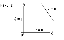
We wish to see projectve plane with lattices like XY-coordinates. But it is impossible.
Fig. 2 is drawn by force. The inclined line = 0 is the straight line at infinity, not a coordinate axis. Well, such a drawing is too much idealistic and of no use.
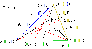
Fig. 3 shows what is called a coordinate triangle. It is constructed with straight lines = 0, = 0 and straight line at infinity = 0. The line at infinity is equally treated without distinguishing from others. Since a point in homogeneous coordinates is defined by a continued ratio : : vertices of the triangle are set as shown. We colored number "0" and sides for easy to see. Point E (1, 1, 1) is the unit point.
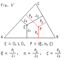
Fig. 3' shows that the homogeneous coordinate of point P is defined by positional relation with the unit point E(1, 1, 1).  and
and  are ordinary distances to each side of triangle ABC. The unit point E can be set anywhere except on sides of triangle ABC, but the homogeneous coordinate of point P changes accordingly.
If point P gets out of triangle ABC over side BC, we change the sign of  to negative. Similarly we do as to
  and
and  . Side AC is the straight line at infinity from the view point of homogeneous coordinates.
Both of Fig. 3 and Fig. 3' do not directly concern to the followings. We just drew them as visual pictures.
By the way, primarily projective geometry has no idea of coordinates. It is a temporary means for our convenience to handle a matter analytically.
**************************************************
 Now we are going to see how the circle of Klein's disk model comes out.
Look at Fig. 4.
Pencils with center O and center O' have four common poins on straight line  as shown. We project them onto straight line a and b. Every red straight line a point on line a and its corresponding point on line b. Seeing the red lines, it is impossible to move the four points on line a to line b by single projection (perspective transformation), like the illustration in dotted box. In order to move the four points on line a to line b, we first move them to line , and then move them from line to line b. In general we have to carry out several perspective transformations to move sequece of points on any straight line onto an optional straight line as corresponding points.
Projective transformation directly moves, as indicated with red thick lines, a point to a point and a straight line to a straight line wthout such a detour.
However, we can not move any three points on a straight line to optional three points on another straight line. Because, when the destination of first two points are settled, that of the third point is automatically fixed as a corresponding point.
Do not forget about that projective transformation is a rule we made. We or nature are not in a position being controlled by projective transformation. We have self-direction.
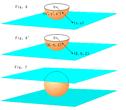
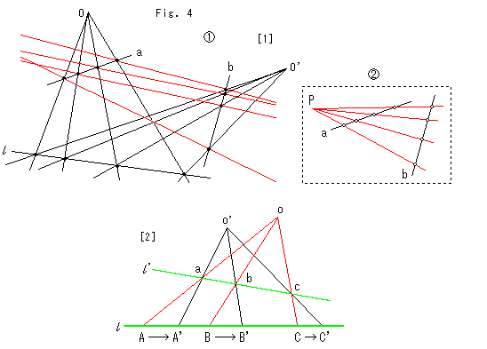
Look at Fig. 5 above. The lattice drawn on the ground is projected to the hemisphere. The hemisphere is set on the ground and its center O is the projection center. Gray straight lines are example of rays
Fig. 6 shows the hemisphere of Fig. 5 with coordinates. The radius of hemisphere is 1.
Let us describe point (x, y) on the sky blue plane in homogeneous coordinates.
 Since
Since


we can use the coordinates (x', y', z') on the hemisphere as homogeneous coordinates on the plane,
= x', = y', = z'.
Fig. 6' shows the hemisphere and plane with new coordinates. (, , ) on the plane is homogeneous coordinates. And (, , ) on the hemisphere is non-homogeneous coordinates. However, we can treat the hemisphere as a projective plane if we regard it as a deformed plane. That is, both the plane and hemisphere are now projective plane. Seeing Fig. 1, it is natural isn't it?
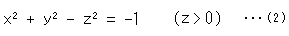
Fig. 7 is a sphere with planes at top and bottom. The hemisphere does not cover the area > 0. So we constructed the sphere instad of the heisphere.
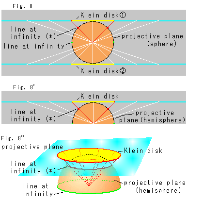
Fig. 8 a cross section that cuts the sphere through its center with planes are leveled. The white lines are rays from the center. We may choose either of the upper plane or the lower. The picture is for the upper plane. We get a circle with the same radius as that of the sphere when we cut the plane with red rays of 45 . We plan to make it Klein's disk. The red spots are on the sphere and correspond to the circumference of circle of Klein's disk
  . We regard the circle on the sphere that goes through the red spots as line at infinity (*) from the view point of Klein's disk . We marked it with (*) because it is what we regarded. Originally the line at infinity on the sphere is the equator that goes through the green spots.
Fig. 8' is the upper half of Fig. 8. We cut away the lower half because we realized that we do not need the full sphere. And the problem of identification of antipodal points of the sphere was melted at the same time. Antipodal points of the disk is not to be identified.
Fig. 8'' is a stereo view of Fig. 8'. Now we cut out the yellow disk with red edge, and we can obtain Klein's disk by metrization.
Be that as it may, it is still questionable. Seeing Fig. 6', any point (, , ) on the plane must meet

(This equation is not a homogeneous expression, so that we can not change it to a non-homogeneous expression.)
Since the left side is constant, we get a quadratic curve
on the plane. It is an imaginary circle with radius  . We will meet this imaginary circle later on. In non-homogeneous coordinates it is
This circle is called an absolute circle in projective geometry. It's strange, isn't it?
Apart from the circle, we feel it intentional that we cut the plane with rays of 45. Let us deside temporarily;
We follow Fig. 6' to get a projective plane.
We use the structure in Fig. 8'' only for cuttig the circle out of the plane.
As a matter of fact, the plane model of elliptic geometry comes out of the absolute circle. But we do not pursue it now.
**************************************************
Now we use an imaginary sphere.
We can smoothly get the disk without cut-out or like. Some mathematicians say "We'll miss real geometry if rely on an imaginary sphere." It is true in a sense. But it is said that hyperbolic geometry comes out of an imaginary sphere. It cause us not to forget about an imaginary sphere.
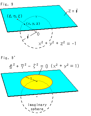 Look at Fig. 9.
The dotted circle represents an imaginary sphere with radius  (=). A sky blue plane is horizontally put on the north pole. Let a point on the sphere be (x, y, z) and its corresponding point on the plane be (, , ). Then, because of imaginary sphere this time,

Wow, imaginary ratio! Anyway as it is, we can write
 Hence
Hence
Needless to say, the left side is on the sphere and the right side is on the (projective) plane.
The left side is invariant wherever point (x, y, z) is on the sphere, so that the right side is invariant. Therefore, a unit circle on the plane
is also invariant. In non-homogeneous coordinates it is

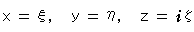
This is an absolute circle, too. But we use it this time. It is a real circle because the right side is positive (real number) and so x and y are real number.
Thus the real unit circle automatically appeared out of the imaginary sphere as shown Fig. 9'. We can make Klein's disk from the circle by metrization. But we are in trouble because the imaginary sphere is invisible.
**************************************************
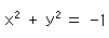
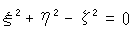
The right side of equation (1) is
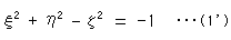 Compare it with a hyperboloid of revolution
They are the same in form, aren't they? We can naturally see the hyperboloid with our own eyes because every letter is real number. Let us regard point (, , ) on the plane as a point (x, y, z) in 3-dimentional cordinates. And we rewrite expressin (1') to expressin (2). Then, the imaginary sphere appears in our site as a hyperboloid.
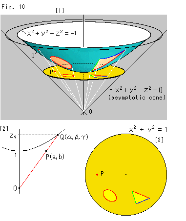 Look at Fig. 10.
[1]: The vertex of asymptotic cone of the appeared hyperboloid was the center of imaginary sphere so that the disk is in contact with the bottom (z = 1) of the appeared hyperboloid as shown. Seeing white rays, point Q never leaves the hyperboloid wherever point P moves in the disk, and similarly point P never gets out of the disk wherever point Q moves on the hyperboloid.
[2]: Let point P be (a,b) and point Q be  . Then

That is, the homogeneous coordinates of a point on the disk equals to the non-homogeneous coordinates of the corresponding point on the hyperboloid. And
We omit to look into distances on the hyperboloid.
[3]: It is the right down view of the disk in [1]. The ellipse is a hyperbolic circle.
There is another way to visualize the imaginary sphere. We pay attention to the left side of equation (1) instead of the right. It is
Now we formally change z into z. Then we get equation (2). The result is the same as above.
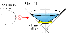
It is quite alright. Marvellous! It's easy to understand. But don't you feel something tricky? Is it allowable to rewrite a character optionally? Should we accept it as a mathematical technique?
Fig. 11 shows a magic. The red snaked arrow indicates to take the form of hyperboloid. We may say that visualized object is a substitute.
Be that as it may, the relation between making the disk and metrization of it is not much clarified. Let us see what is called group. We may find something new.
[Back] [Next] [Contents]